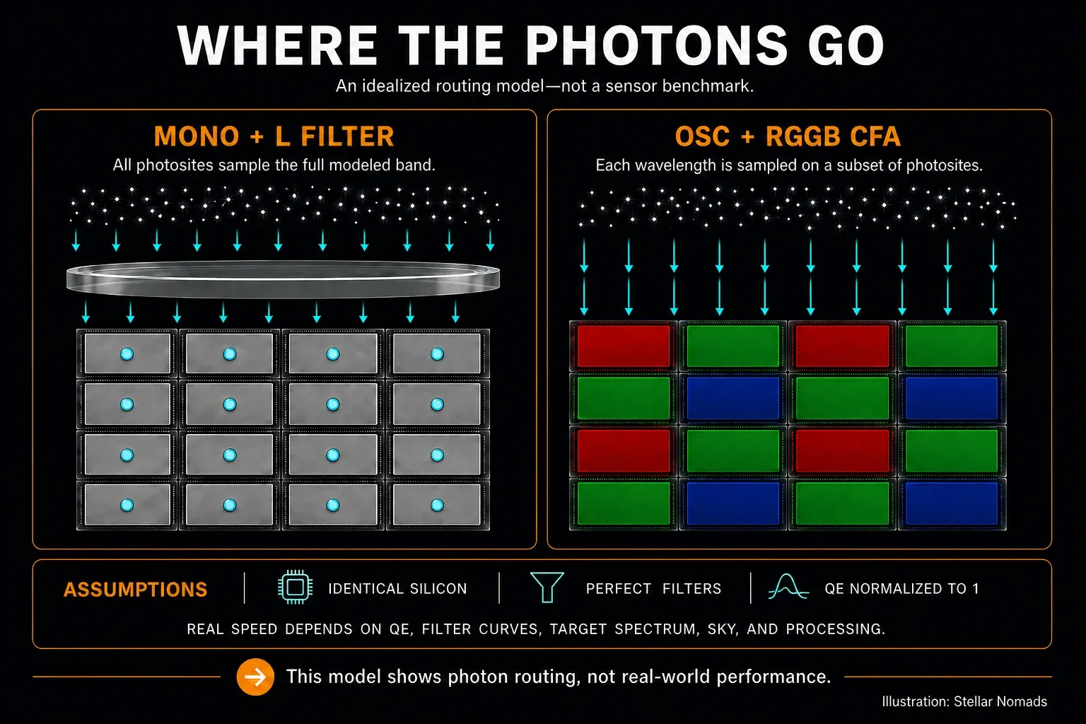
In mono vs color astrophotography, there is no universal speed multiplier. Under a deliberately ideal broadband-luminance model, mono accepts three times as many wavelength-matched samples. Real exposure time also depends on quantum efficiency, filter curves, target spectrum, sky brightness, read noise, sampling, and how the data will be processed.
The simulator above demonstrates the narrow claim that Bayer geometry can support. It sends the same idealized photon stream to identical silicon, exposes every assumption, and counts accepted samples. It is a thought experiment, not measured camera data and not a promise that one system will finish a real image three times sooner.
That distinction matters. The original version of this comparison mixed model output with unverified device-like values. This revision removes that sensor mode and separates three questions that are often collapsed into one: where photons are routed, how those photons affect signal-to-noise ratio, and how quickly a finished image can be produced.
What actually differs between mono and OSC sensors?
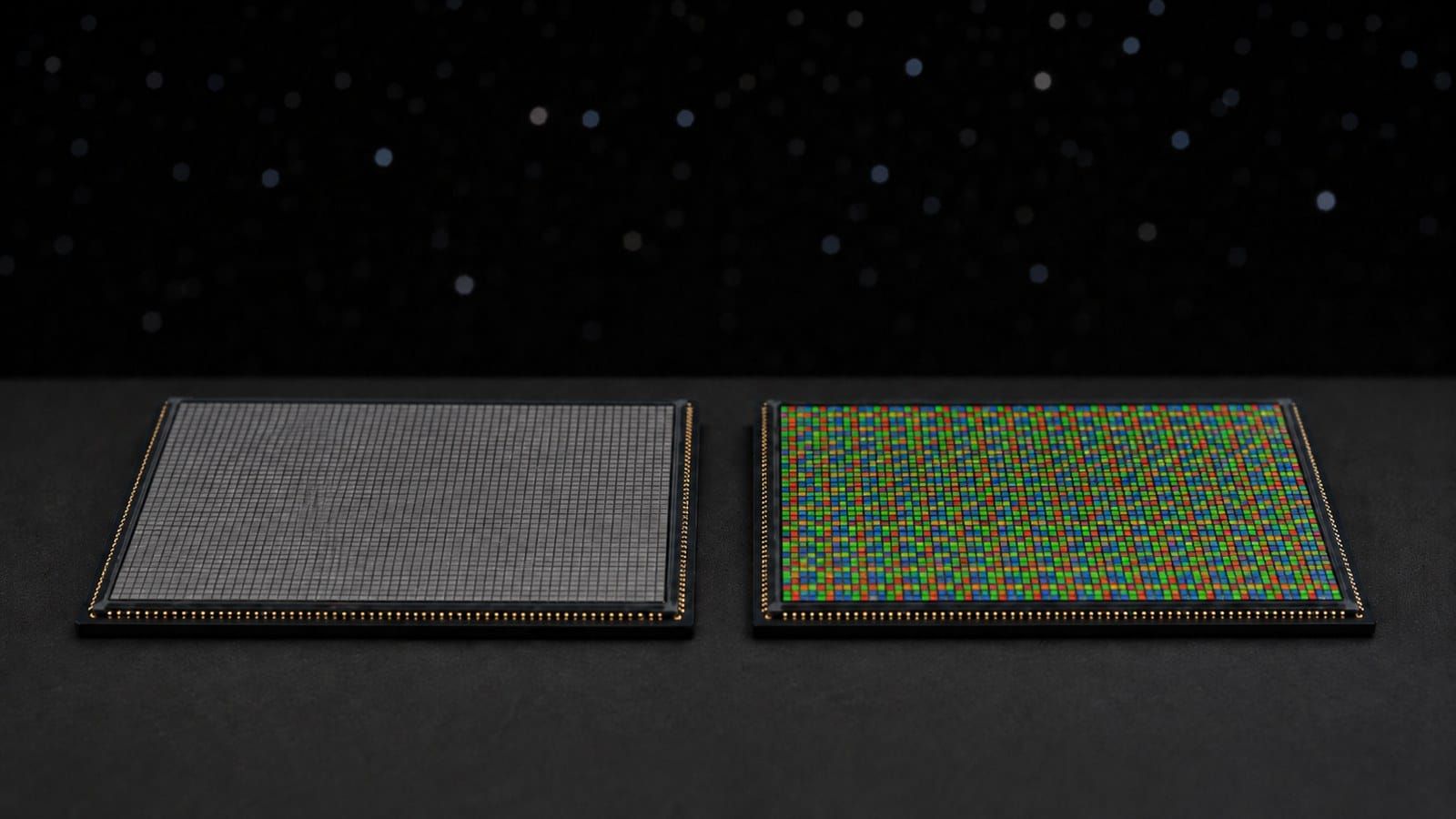
The visible difference is where color selection happens. A monochrome astronomy camera has no Bayer color-filter array over its photosites. For color imaging, an external filter selects a band for the entire sensor. A one-shot-color camera has a repeating red-green-green-blue, or RGGB, filter pattern over the sensor, so neighboring photosites sample different spectral bands in the same exposure.
Both arrangements discard light. A real luminance filter is not perfectly transparent, and real red, green, and blue filters do not have vertical edges. Bayer dyes also transmit less than 100%, overlap spectrally, and behave differently with wavelength. The detector's own quantum efficiency changes across the spectrum as well.
That is why “mono records all the light” and “OSC records exactly one third” are too broad as real-camera statements. They can describe one normalized geometry model, but neither sentence is a measured throughput specification. The word all must mean all photons accepted by the model, not all photons that entered a telescope.
Scientific observatories use monochrome detectors and external filters for the same basic reason: each exposure can be assigned to a defined band, then combined later. NASA’s current explainer on light passing through a Hubble filter shows that architecture without implying that its throughput is perfect.
What can the simulator prove?
It proves only the arithmetic of an idealized routing model. The model assumes identical silicon, quantum efficiency normalized to one, perfect non-overlapping filters, equal red, green, and blue photon rates, no sky background, no read noise, and no processing. Every result must remain attached to those assumptions.
In the broadband-luminance mode, the mono side accepts every modeled red, green, and blue photon because its ideal luminance passband includes all three. The OSC side accepts a photon only when its wavelength label matches the idealized dye over the photosite it hits. With an RGGB tile and an equal mix of red, green, and blue photons, the expected accepted fraction is one third.
That produces a three-to-one ratio in accepted modeled samples. It does not by itself produce a three-to-one ratio in real system throughput, spatial resolution, signal-to-noise ratio, or completed-image speed. Those are different quantities.
The equal-time RGB mode makes the boundary clearer. If a mono system divides its total time equally among ideal red, green, and blue filters, it accepts one matching band for one third of the schedule. The OSC system observes all three bands continuously, but each photon is accepted only at a matching photosite. In this flat-spectrum idealization, both sides accept one third of the incident stream on average.
This equality does not mean the images are identical. The mono system obtains a complete photosite grid for each filter exposure, while OSC data must be reconstructed from the mosaic. Dithering, registration, drizzle, demosaicing, optical sampling, seeing, and the final color workflow all affect what detail survives.
How does a luminance-heavy schedule change the ideal ratio?
Within the same ideal model, the accepted-sample ratio is set by the fraction of mono time assigned to luminance. Let f be that fraction. Mono accepts a normalized rate of one during luminance and one third during RGB time; OSC accepts one third throughout. Dividing those rates gives a simple result: ratio = 1 + 2f.
| Modeled schedule | Luminance fraction | Derived ratio |
|---|---|---|
| L only | 1 | 3.00:1 |
| 8:1:1:1 LRGB | 8/11 | 2.45:1 |
| 4:1:1:1 LRGB | 4/7 | 2.14:1 |
| 1:1:1:1 LRGB | 1/4 | 1.50:1 |
| 1:1:1 RGB, no L | 0 | 1.00:1 |
These numbers are derived from the stated assumptions, not measurements from a named camera. Change the source spectrum, filter transmission, or detector response and the ratios change. Even within broadband imaging, stars, reflection nebulae, galaxies, airglow, and artificial light do not provide the equal RGB photon stream used by the model.
The table is still useful. It shows why a blanket phrase such as “mono is twice as fast” hides the most important decision: how much high-quality luminance will actually be used in the final image. A workflow built around a deep luminance stack is not the same experiment as a workflow built around equal RGB integration.
How do photon counts become exposure time?
They do not convert through one universal rule. In a source-shot-noise-limited thought experiment, signal-to-noise ratio grows with the square root of detected signal. If a system detects photons at three times the rate and every other condition is identical, it reaches the same photon count in one third of the time and achieves the square root of three times the shot-noise-limited signal-to-noise ratio in equal time.
Real imaging usually includes sky background. If signal and background are both reduced by the same throughput factor, the familiar inverse-throughput time scaling can still appear in a background-limited approximation. But a Bayer array and an external filter set do not necessarily scale target signal and sky background by the same factor at every wavelength. A sodium-rich sky, moonlight, continuum emission, and a narrow spectral line each interact differently with the passbands.
Read noise adds another dependency. The cost depends on the number and duration of sub-exposures, the camera's read noise at the chosen gain, and the background electrons accumulated per photosite. A “ratio squared” rule is not universal: it describes a restricted case where signal rate changes while fixed read-noise variance and sub-exposure cadence are held constant. Change the cadence or reach the background-limited regime and the scaling changes.
Use the sub-exposure calculator to test whether a planned sub-exposure is long enough for the sky background to dominate read noise. Use the integration time calculator for signal-to-noise planning, but enter values derived from your own equipment and sky rather than substituting the ideal ratio from this page.
What changes on real cameras?
A real comparison needs wavelength-dependent data, not a single peak-QE number. ZWO lists a peak quantum efficiency of 91% for the ASI2600MM Pro and 80% for the ASI2600MC Pro on its official ASI2600 product page. Those are useful manufacturer specifications. They are not full spectral-response curves, and the ratio 80/91 should not be applied as a wavelength-independent transmission correction.
For a defensible device-specific model, the required inputs are the mono and color spectral-response curves at the operating mode, transmission curves for every external filter, telescope throughput, the target spectrum, and local sky spectrum. The model should also identify whether published color-camera QE already includes the Bayer array, or it risks charging the same loss twice.
Published research can help characterize general camera sensitivities. The EPFL spectral-sensitivity database reports measurements for 28 cameras, and a later MNRAS study used camera sensitivity functions in an astronomy context. Such population data can illustrate how dyes overlap. It cannot substitute for a measured response curve from the exact astronomy camera being compared.
Sampling matters too. A mono exposure records one filtered value at every photosite. An OSC exposure records one color-filtered value at each photosite and estimates the missing color components during demosaicing. How much practical detail that costs depends on the optical point-spread function, seeing, pixel scale, dither pattern, reconstruction method, and whether the data are drizzled.
Modern CMOS binning also needs careful wording. Many astronomy cameras combine pixels digitally rather than performing charge-domain hardware binning in the CCD sense. The consequences depend on the camera and software path. Our guide to camera binning covers that distinction, while the pixel-scale guide helps determine whether either camera is over- or undersampling the optics.
What happens in narrowband?
Narrowband cannot be reduced to the broadband one-third result. A line occupies a narrow wavelength region, and the response of each Bayer dye at that wavelength determines which photosites contribute and by how much. The ideal simulator's H-alpha mode deliberately assumes zero dye leakage: every mono photosite responds, while only the red photosites in an RGGB tile respond. That creates a four-to-one accepted-sample ratio inside that artificial model.
A real H-alpha result requires the red, green, and blue spectral-response values near 656.3 nm. A real OIII result requires those values near 500.7 nm. The location of OIII near overlapping green and blue responses makes generic claims especially risky. Without the exact camera's curves, the direction and size of an OIII advantage are unknown.
Duoband filters give OSC a genuine scheduling benefit: two line regions can be recorded in one exposure. Mono normally records one narrow band at a time. But simultaneous collection does not automatically mean that both reconstructed line channels have equal throughput, equal spatial sampling, or clean separation.
H-alpha and SII both occupy the red end of the visible spectrum. When a single OSC exposure passes both lines into the same red-filtered photosites, the image does not contain enough information to assign each detected electron uniquely to one line. Separate filter combinations or additional assumptions are needed. Filters such as Optolong's L-Synergy, which passes OIII and SII, are designed to pair with another dual-band filter as part of a multi-exposure workflow.
Does a 3 nm filter automatically beat a 7 nm filter by 1.5×?
No; that figure belongs to a specific approximation. If both filters have the same line transmission, the target line is much narrower than either passband, the sky spectrum is flat across both bands, and the exposure is background-limited, sky background scales with bandwidth. The signal-to-noise ratio then scales approximately with the inverse square root of bandwidth. Under those assumptions, the ratio is √(7/3), or about 1.53.
Real filters can differ in peak transmission, band shape, central-wavelength shift in fast optical systems, out-of-band blocking, and halo behavior. Real sky spectra are not flat. The square-root calculation is therefore a useful conditional estimate, not a general product ranking.
Which workflow should you choose?
Choose the workflow whose constraints match your sky time and science or imaging goal. OSC reduces hardware, calibration branches, filter changes, and the risk that a short clear window ends before every color channel is complete. It can produce a usable color dataset in one session and works well with carefully chosen dual-band filters.
Mono provides direct control over each passband. It is the stronger choice when separate calibrated channels, full-grid samples through each filter, flexible exposure weighting, or clean H-alpha/OIII/SII separation are central requirements. The cost is a filter wheel or manual changes, more calibration sets, per-filter focus management, and a larger automation surface.
For broadband aesthetic imaging, ask how much luminance you will truly collect and use. For narrowband, ask whether line separation matters more than simultaneous acquisition. For variable weather, count completed datasets rather than theoretical photons. For photometry or other measurement work, define the required passband and calibration method before choosing a color architecture.
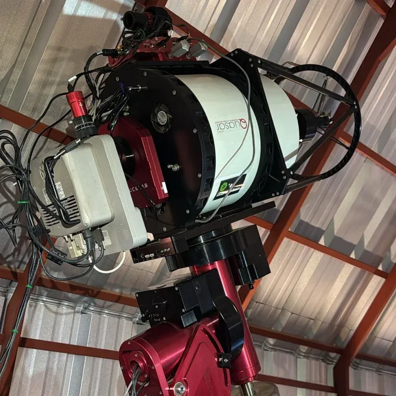
Our Deepsky Chile rig uses mono because reliable automation and repeated sky access make the added channel management worthwhile. That is a workflow-specific choice, not evidence that every imager should choose the same architecture.
Frequently asked questions
Is a mono camera twice as fast as OSC?
No universal multiplier applies. An idealized luminance-routing model gives a three-to-one accepted-sample ratio, while an equal-time RGB model gives one-to-one. Real exposure time depends on spectral response, filters, target, sky, noise, sampling, and processing.
Does mono always produce better image quality?
Mono records a complete photosite grid through each external filter, while OSC reconstructs missing color components from a mosaic. Whether the visible difference is important depends on seeing, optics, pixel scale, dithering, reconstruction, integration, and output size.
Can an OSC camera do narrowband imaging?
Yes. Dual-band and multi-band filters make OSC narrowband practical and allow simultaneous collection of selected line regions. Throughput and line separation remain wavelength- and filter-dependent, so use measured curves for a specific comparison.
Do I need a filter wheel for a mono camera?
Not for greyscale imaging or manual single-filter work. An automated multi-filter color or narrowband program usually benefits greatly from a filter wheel because it can sequence filters repeatably without manual intervention.
Is mono worth it for a beginner?
It depends on the beginner's goal and tolerance for complexity. OSC shortens the path to a complete color dataset. Mono offers more passband control but adds filters, calibration branches, focusing considerations, and sequencing.
Do peak-QE specifications settle the comparison?
No. Peak QE is one value at or near one wavelength. A valid exposure model needs the response across the wavelengths of interest, plus filter transmission, target and sky spectra, noise settings, and the acquisition schedule.