Quantum efficiency in astronomy cameras is one of the most quoted numbers on a spec sheet — and one of the most misunderstood. When you compare two cooled cameras and one boasts 91% quantum efficiency against another's 55%, it is tempting to assume the first is nearly twice as good at everything. The reality is more interesting, and far more useful to understand before you spend money.
Quantum efficiency (QE) in astronomy cameras is the percentage of incoming photons a sensor converts into a measurable electrical signal. A camera at 90% QE records almost every photon that reaches it; one at 50% throws half of them away. Higher QE means more signal, better reach on faint targets, and shorter exposures — but it is only one part of what makes an image.
This guide is written for imagers choosing or comparing a camera — whether it is your first cooled astro-camera or a narrowband upgrade for an existing rig. We will keep the physics plain, put real numbers on it, and be honest about where QE genuinely moves the needle and where it quietly does not. Everything here builds on the wider set of astrophotography fundamentals that decide how clean your final image looks.
What is quantum efficiency in a camera?
Quantum efficiency is the fraction of photons landing on a sensor that get turned into signal, written as a percentage. If 100 photons of a given colour strike a pixel and the sensor registers 60 of them, its quantum efficiency at that wavelength is 60%.
That is the whole idea. A perfect detector would count every photon and have 100% QE. No real sensor does, because some photons reflect off the surface, some pass straight through the silicon without being absorbed, and some are absorbed in the wrong place and never counted. QE simply measures how good the sensor is at catching and keeping the light that arrives.
In astrophotography this matters more than in daytime photography, because the targets are faint. A galaxy or a dim emission nebula delivers only a trickle of photons per pixel per second. Waste half of them and you either need twice the exposure to reach the same result, or you accept a noisier image. That is why QE sits near the top of the spec list for any serious deep-sky camera.
How quantum efficiency actually works
Inside every astronomy camera — CCD or CMOS — each pixel is a tiny light bucket built from silicon. When a photon is absorbed, it frees an electron through the photoelectric effect. The camera counts those electrons, converts the count to a number, and that number becomes the brightness of one pixel. Quantum efficiency is the link between the photons that arrive and the electrons the sensor actually collects:
QE = (electrons collected) ÷ (photons that arrived) × 100%
So a sensor with 80% QE that is hit by 1,000 photons produces about 800 electrons of signal. The same 1,000 photons on a 40% sensor yield only 400 electrons. Same telescope, same sky, same target — half the signal, purely because of the detector.
One subtlety worth holding onto: QE describes how efficiently photons become signal electrons. It says nothing about the noise the camera adds on top. A high-QE sensor with sloppy read noise can still be beaten by a slightly lower-QE sensor that is much quieter. We come back to that trade-off below, because it is where a lot of buying decisions go wrong.
Why quantum efficiency matters for astrophotography
The reason QE earns its place is signal-to-noise ratio (SNR) — the single number that decides whether faint detail survives or drowns in grain. More collected photons means more signal, and because the random shot noise of light grows only as the square root of the signal, more signal always improves SNR.
Put practically, higher quantum efficiency buys you three things:
- Reach. Faint outer galaxy arms, dim tidal streams, and weak nebulosity climb above the noise sooner.
- Time. A sensor with roughly double the QE reaches the same SNR in roughly half the total integration — a real gift when clear nights are rare.
- Flexibility. Shorter usable sub-exposures ease the demands on tracking, and make the most of the light that does get through when you are shooting under light-polluted skies.
That said, QE is a multiplier on the light your optics already deliver. A high-QE camera on a small aperture under a bright sky still collects fewer photons than a modest camera on a large aperture under dark skies. The detector is one link in a chain that runs from aperture and sky quality through the optical train to the sensor.
Why quantum efficiency changes with wavelength
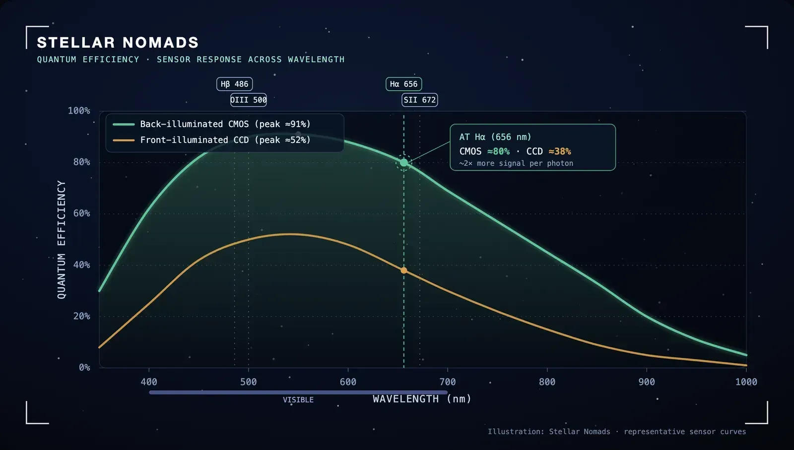
Here is the detail most spec sheets hide behind a single headline figure: quantum efficiency is not one number. It changes with the colour of the light. Silicon absorbs green and red light readily but struggles with deep blue and ultraviolet, and becomes increasingly transparent to near-infrared. So every sensor has a quantum efficiency curve, usually peaking somewhere in the 500–600 nm range and falling off toward both ends of the spectrum.
For broadband imaging this mostly averages out. For narrowband imaging it is decisive. Emission nebulae glow at specific wavelengths — hydrogen-alpha (Hα) at 656 nm, doubly ionised oxygen (OIII) at 500/501 nm, and sulphur-II (SII) at 672 nm. If you shoot Hα, the only QE that matters to you is the sensor's efficiency at 656 nm, not its glossy peak figure at 550 nm.
This is why two cameras quoting the same peak QE can perform differently on the same target. A sensor that holds 80% at 656 nm will pull in far more Hα signal than one that peaks at 90% but has already dropped to 55% by the red end. When you compare cameras for narrowband work on emission nebulae, read the curve at your wavelengths, not the headline.
Front-illuminated vs back-illuminated sensors
The biggest single jump in astronomy-camera QE over the past decade did not come from a new kind of silicon — it came from turning the chip around — the move to the back illuminated sensor (BSI), which we unpack in its own guide. Understanding this is the key to reading a modern camera's QE figure, so it is worth a close look at how a pixel is actually built.
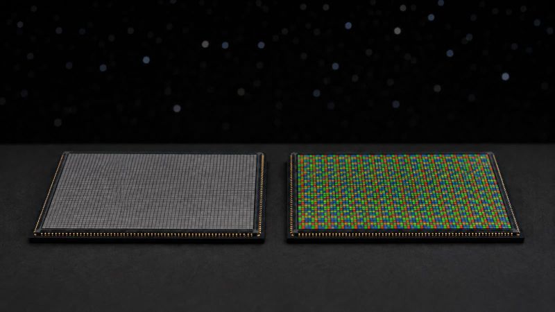
In a front-side illuminated (FSI) pixel, the metal wiring and transistors sit on the same surface that faces the sky. That metal is opaque, so it does not gently dim the light — it blocks part of the pixel outright, and photons only reach the silicon through the gaps between the wiring. Tiny microlenses on top help by funnelling light into those gaps, but a real fraction of each pixel is still shadowed. The share of the pixel that actually collects light is called the fill factor, and for FSI sensors it is often only around 40–60%. Blue and ultraviolet light suffers most, because it is absorbed in the overlying gate and filter layers before it ever reaches the photodiode.
A back-side illuminated (BSI) sensor is literally flipped over, and the silicon is ground down to a few microns thick, so light now enters from the back and lands directly in the photodiode across almost the whole pixel — a fill factor close to 100%, with the wiring tucked safely behind. Add an anti-reflection coating to that newly exposed back surface and short-wavelength response improves as well. Together these lift representative peak QE from roughly 55–80% (FSI) to about 90–95% (BSI) — a little over half a stop of extra signal. Note the word "together": the gain comes from back-illumination plus newer manufacturing and better coatings, not from flipping the chip alone.
Two honest caveats keep this straight. First, back-illumination is not the same thing as CMOS — it is an independent design choice, and top scientific CCDs have been back-illuminated for decades. So BSI is not what makes CMOS "beat" CCD; CMOS wins on read noise, speed, and cost, which we come to next. Second, thinning the silicon boosts blue and visible QE but can actually reduce deep-red and near-infrared response, because long-wavelength photons need thicker silicon to be absorbed. Sensors chasing strong red or NIR use thicker "deep-depletion" silicon rather than simply going thin — another reason to read a QE curve at the wavelengths you actually shoot, not just its peak.
A note on blooming. You will sometimes see "blooming" raised alongside sensor design, but it is a separate matter from QE and illumination. Blooming happens after photons become electrons: when a very bright star fills a pixel's well to capacity, the excess charge spills into its neighbours and paints a bright streak. That is about full-well depth and anti-blooming gates, not about how efficiently the pixel captured light in the first place — so a high-QE sensor is no more or less prone to it. It belongs to the dynamic-range side of the spec sheet, and it does not change how you read a QE curve.
CCD vs CMOS quantum efficiency
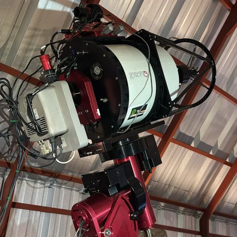
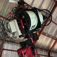
For decades, cooled CCDs were the gold standard for scientific and deep-sky imaging, and the best of them reached respectable QE. Our own remote rig at Deepsky Chile — an SBIG STL-11000 built around a large Kodak KAI-11000 CCD — sits right in that older front-illuminated class, with a peak QE near 50%. It has captured beautiful data under Bortle 1 Atacama skies for years, which is a useful reminder that QE is not destiny.
Modern back-illuminated CMOS sensors have simply moved the ceiling. A current mono camera built on the Sony IMX455 or IMX571 reaches roughly 90–91% at peak — close to double the photon capture of that legacy CCD at the same wavelength. Combined with much lower read noise and no need for the fast mechanical shutter a CCD demands, CMOS has become the default for new deep-sky rigs. The frontier keeps moving, too: NASA is developing single-photon-sensing CMOS detectors for future space telescopes hunting for signs of life on distant worlds.
| Sensor | Detector type | Class | Approx. peak QE |
|---|---|---|---|
| Sony IMX455 / IMX571 | CMOS, back-illuminated | Modern mono & colour | ~90–91% |
| Sony IMX533 / IMX294 | CMOS, back-illuminated | Modern colour | ~90% |
| Sony ICX694 | CCD, front-illuminated | Older high-QE CCD | ~76% |
| Kodak / ON KAI-11000 | CCD, front-illuminated | Legacy large CCD | ~50% |
These are manufacturer peak figures, measured at the sensor's best wavelength and usually for the monochrome version. A one-shot-colour (OSC) camera using the same chip effectively delivers lower QE per channel, because its Bayer colour filters absorb light before it reaches the pixel — the trade you accept for capturing colour in a single exposure. We put numbers on that trade-off in our full mono vs OSC speed comparison.
How much does quantum efficiency really matter?
This is the honest part. Quantum efficiency is important, but it suffers from steep diminishing returns, and it is easy to over-weight it against factors that matter more.
Consider the numbers. Going from a 50% sensor to a 90% sensor is a genuine 1.8× jump in captured signal — worth chasing. But going from 85% to 91% is only about a 7% gain, which under real skies is often lost in the noise of everything else. Once you are already in the high-80s, extra QE is a rounding error, not a revolution.
Meanwhile, several other things swing your result far more than that last few percent of QE:
- Sky darkness. Moving from a bright suburban sky to a truly dark site can improve SNR more than any sensor swap.
- Aperture and total integration time. More collecting area and more hours on target beat a marginal QE upgrade almost every time.
- Read noise and thermal noise. A quiet, well-cooled sensor with clean calibration frames preserves the faint signal that a noisy sensor buries — regardless of headline QE.
- Sampling. Getting your pixel scale matched to the seeing and your resolution right protects detail that no amount of QE can recover once it is lost.
So treat QE as a tie-breaker, not a trophy. When two cameras are otherwise close, prefer the higher QE — especially at your working wavelengths. But do not pay a large premium to climb from 88% to 91%, and never let a high QE figure distract you from read noise, cooling, pixel size, and the sky above your telescope.
How to read a camera's QE spec
When you sit down to compare cameras, a few habits keep you honest:
- Find the curve, not just the peak. A reputable manufacturer publishes a QE-versus-wavelength graph. Read it at the wavelengths you actually image — 656 nm if you shoot Hα, the blue-green region if you chase OIII galaxies and planetary nebulae.
- Check whether the figure is mono or colour. A "91% QE" claim almost always refers to the monochrome sensor. The colour version of the same chip captures less per channel.
- Be sceptical of absolute-vs-relative curves. Some plots are normalised so the peak reads 100% (relative QE). That tells you the shape of the response but not the true photon-capture efficiency. Look for absolute QE in percent.
- Weigh QE against the rest of the spec. Read noise in electrons, full-well capacity, pixel size, and cooling delta all belong in the same decision.
Get into that habit and the marketing headline stops steering you. You start choosing the camera that collects the most of your light, cleanly — which is the whole point of caring about quantum efficiency in the first place.
Frequently asked questions about quantum efficiency
What is a good quantum efficiency for an astronomy camera?
For a modern deep-sky camera, a peak QE in the mid-80s to low-90s percent is excellent and typical of current back-illuminated CMOS sensors. Anything above about 80% at your working wavelength is very good. Older or budget sensors in the 50–65% range still take fine images; they simply need more integration time to match the reach of a high-QE sensor.
Is higher quantum efficiency always better?
All else being equal, yes — more captured photons is always an advantage. But all else is rarely equal. A camera with slightly lower QE but much lower read noise, better cooling, or a more suitable pixel size can produce a better final image. QE is one factor among several, and it shows steep diminishing returns above roughly 85%.
Do CMOS cameras have higher quantum efficiency than CCD?
Modern back-illuminated CMOS sensors generally do, reaching around 90% versus the 50–77% of most CCDs. The gap comes mainly from back-illumination and modern manufacturing rather than from CMOS versus CCD as such. A few late high-end CCDs reached the mid-70s, but current CMOS sensors combine high QE with far lower read noise, which is why they now dominate deep-sky imaging.
Does quantum efficiency matter more than pixel size?
Not usually. Pixel size, together with your telescope's focal length, sets your sampling and how well you match the seeing — and mismatched sampling throws away detail that high QE cannot recover. Think of QE as improving how much signal you collect, and pixel size as improving how well you resolve it. Both matter; for most rigs, getting sampling right comes first.
Does a light-pollution filter reduce quantum efficiency?
A filter does not change the sensor's QE, but it does block some wavelengths before they reach the sensor, so the effective signal you collect drops in those bands. That is a deliberate trade: you lose some broadband light in exchange for far better contrast on emission targets under bright skies. The sensor is still converting photons at its rated QE — there are just fewer photons getting through.
How is quantum efficiency measured?
Manufacturers illuminate the sensor with a calibrated light source of known photon flux at each wavelength and compare the electrons produced to the photons delivered. The result is the absolute QE curve you see on a datasheet. Because it depends on wavelength, temperature, and sometimes bias conditions, published figures are best treated as representative rather than exact.
The bottom line
Quantum efficiency tells you how much of the light your telescope delivers actually becomes signal — and modern back-illuminated sensors have pushed that from around half to nearly all of it. That is a real, worthwhile gain, and it is smart to prefer a higher-QE camera when the rest of the spec is close, especially at the narrowband wavelengths you image most.
But QE is a multiplier, not a miracle. Dark skies, aperture, integration time, read noise, and correct sampling all shape your final image at least as much as the last few percent of quantum efficiency. Understand the curve, read it at your wavelengths, and let it inform your choice without letting it dominate it. For the next step, see how the detector fits into the full imaging chain in our guide to astrophotography fundamentals, and how long exposures earn that signal in our walkthrough of autoguiding.